How to pick a random number from 1-10
Imagine you have to generate a uniform random number from 1 to 10. That is, an integer from 1 to 10 inclusive, with an equal chance (10%) of selecting each one. But, let’s say you have to do this without access to coins, computers, radioactive material, or other such access to traditional (pseudo) random number generators. All you have is a room of people.
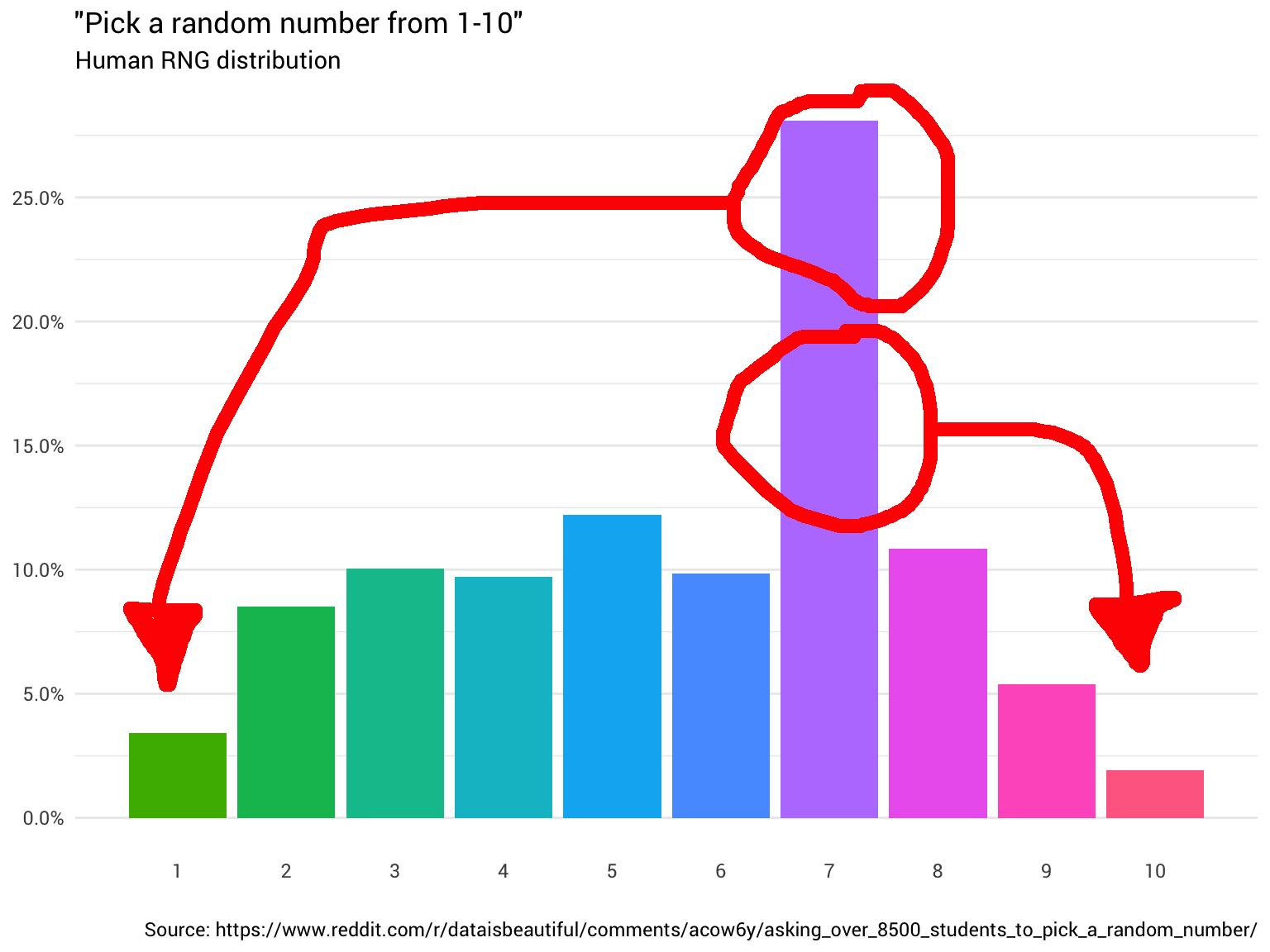
For the sake of argument, let’s say this room has a little over 8500 students in it.
The easy thing to do is to ask someone “Hey, pick a random number from 1 to 10!”. The person replies “7!”. Great! Now you have a number. However, you start to wonder, is the number uniformly random?
So you decide to ask a few more people. You continue to ask people and count their responses, rounding non-integers and ignoring answers from people who think that 1 to 10 includes 0. Eventually you start to see that the pattern is not flat at all:
library(tidyverse)

probabilities <-
  read_csv("https://git.io/fjoZ2") %>%
  count(outcome = round(pick_a_random_number_from_1_10)) %>%
  filter(!is.na(outcome),
         outcome != 0) %>%
  mutate(p = n / sum(n))

probabilities %>%
  ggplot(aes(x = outcome, y = p)) +
  geom_col(aes(fill = as.factor(outcome))) +
  scale_x_continuous(breaks = 1:10) +
  scale_y_continuous(labels = scales::percent_format(),
                     breaks = seq(0, 1, 0.05)) +
  scale_fill_discrete(h = c(120, 360)) +
  theme_minimal(base_family = "Roboto") +
  theme(legend.position = "none",
        panel.grid.major.x = element_blank(),
        panel.grid.minor.x = element_blank()) +
  labs(title = '"Pick a random number from 1-10"',
       subtitle = "Human RNG distribution",
       x = "",
       y = NULL,
       caption = "Source: https://www.reddit.com/r/dataisbeautiful/comments/acow6y/asking_over_8500_students_to_pick_a_random_number/")
Data originally from reddit
You kick yourself. Of course it’s not uniformly random. After all, you can’t trust people.
So, what to do?
What if we could find some function that transforms the “Human RNG” distribution above into a unform distribution?
The intuition for this is relatively simple. All we want to do is move the probability mass where the bars are larger than 10%, and move it to the bars where they are less than 10%. You can imagine this like chopping and reaarranging the bars such that they are all level:
Extending this intuition, we can see that such a function should exist. In fact, there should be many different functions (re-arrangements). To take an extreme example, say we “cut” each bar into infinitesimally small blocks, then we could use these blocks to build up the distribution in whatever shape we wanted (like Lego).
Of course, such an extreme example is a bit cumbersome. Ideally we want to preserve as much of the initial distribution (i.e. do as little chopping and changing) as possible.
How do you find such a function?
Well, our explanation above is beginning to sound a lot like linear programming. To crib from Wikipedia:
Linear programming (LP, also called linear optimization) is a method to achieve the best outcome … in a mathematical model whose requirements are represented by linear relationships. … Standard form is the usual and most intuitive form of describing a linear programming problem. It consists of the following three parts:
- A linear function to be maximized
- Problem constraints of the following form
- Non-negative variables
We can formulate our redistribution problem problem in a similar way.
Representing the problem
We have a set of variables, \(x_{i,j}\), where each one encodes the proportion of probability redistributed from integer \(i\) (1 to 10) to integer \(j\) (1 to 10). So if \(x_{7,1} = 0.2\), then we would need to turn 20% of the responses that are “7” into a “1”, instead.
variables <-
  crossing(from = probabilities$outcome,
           to   = probabilities$outcome) %>%
  mutate(name = glue::glue("x({from},{to})"),
         ix = row_number())

variables
## # A tibble: 100 x 4
## from to name ix
## <dbl> <dbl> <glue> <int>
## 1 1 1 x(1,1) 1
## 2 1 2 x(1,2) 2
## 3 1 3 x(1,3) 3
## 4 1 4 x(1,4) 4
## 5 1 5 x(1,5) 5
## 6 1 6 x(1,6) 6
## 7 1 7 x(1,7) 7
## 8 1 8 x(1,8) 8
## 9 1 9 x(1,9) 9
## 10 1 10 x(1,10) 10
## # … with 90 more rowsWe want to constrain these variables such that the redistributed probabilies all sum to 10%. In other words, for each \(j\) in 1 to 10:
\[ x_{1, j} + x_{2, j} + \ldots\ x_{10, j} = 0.1 \]
We can represent these constraints as a list of arrays in R. Later we will bind them together into a matrix.
fill_array <- function(indices,
                       weights,
                       dimensions = c(1, max(variables$ix))) {
  init <- array(0, dim = dimensions)

  if (length(weights) == 1) {
    weights <- rep_len(1, length(indices))
  }

  reduce2(indices, weights, function(a, i, v) {
    a[1, i] <- v
    a
  }, .init = init)
}

constrain_uniform_output <-
  probabilities %>%
  pmap(function(outcome, p, ...) {
    x <-
      variables %>%
      filter(to == outcome) %>%
      left_join(probabilities, by = c("from" = "outcome"))

    fill_array(x$ix, x$p)
  })
We also have to make sure that all the probability mass from the original distribution is conserved. So for each \(j\) in 1 to 10:
\[ x_{i, 1} + x_{i, 2} + \ldots\ x_{i, 10} = 1.0 \]
one_hot <- partial(fill_array, weights = 1)

constrain_original_conserved <-
  probabilities %>%
  pmap(function(outcome, p, ...) {
    variables %>%
      filter(from == outcome) %>%
      pull(ix) %>%
      one_hot()
  })
And as we said earlier, we want to maximise the amount of the original distribution that we conserve. This is our objective:
\[ maximise (x_{1, 1} + x_{2, 2} + \ldots\ x_{10, 10}) \]
maximise_original_distribution_reuse <-
  probabilities %>%
  pmap(function(outcome, p, ...) {
    variables %>%
      filter(from == outcome,
             to == outcome) %>%
      pull(ix) %>%
      one_hot()
  })

objective <- do.call(rbind, maximise_original_distribution_reuse) %>% colSums()
We can then pass this problem to a solver, like the lpSolve package in R, combining the constraints we have created into a single matrix:
# Make results reproducible...
set.seed(23756434)

solved <- lpSolve::lp(
  direction    = "max",
  objective.in = objective,
  const.mat    = do.call(rbind, c(constrain_original_conserved, constrain_uniform_output)),
  const.dir    = c(rep_len("==", length(constrain_original_conserved)),
                   rep_len("==", length(constrain_uniform_output))),
  const.rhs    = c(rep_len(1, length(constrain_original_conserved)),
                   rep_len(1 / nrow(probabilities), length(constrain_uniform_output)))
)

balanced_probabilities <-
  variables %>%
  mutate(p = solved$solution) %>%
  left_join(probabilities,
            by = c("from" = "outcome"),
            suffix = c("_redistributed", "_original"))
This returns the following re-distribution:
library(gganimate)

redistribute_anim <-
  bind_rows(balanced_probabilities %>%
            mutate(key   = from,
                   state = "Before"),
            balanced_probabilities %>%
            mutate(key   = to,
                   state = "After")) %>%
  ggplot(aes(x = key, y = p_redistributed * p_original)) +
  geom_col(aes(fill = as.factor(from)),
           position = position_stack()) +
  scale_x_continuous(breaks = 1:10) +
  scale_y_continuous(labels = scales::percent_format(),
                     breaks = seq(0, 1, 0.05)) +
  scale_fill_discrete(h = c(120, 360)) +
  theme_minimal(base_family = "Roboto") +
  theme(legend.position = "none",
        panel.grid.major.x = element_blank(),
        panel.grid.minor.x = element_blank()) +
  labs(title = 'Balancing the "Human RNG distribution"',
       subtitle = "{closest_state}",
       x = "",
       y = NULL) +
  transition_states(
    state,
    transition_length = 4,
    state_length = 3
  ) +
  ease_aes('cubic-in-out')

animate(
  redistribute_anim,
  start_pause = 8,
  end_pause = 8
)
Great! We now have a redistribution function. Let’s take a closer/slower look at where exactly the mass is going:
balanced_probabilities %>%
  ggplot(aes(x = from, y = to)) +
  geom_tile(aes(alpha = p_redistributed, fill = as.factor(from))) +
  geom_text(aes(label = ifelse(p_redistributed == 0, "", scales::percent(p_redistributed, 2)))) +
  scale_alpha_continuous(limits = c(0, 1), range = c(0, 1)) +
  scale_fill_discrete(h = c(120, 360)) +
  scale_x_continuous(breaks = 1:10) +
  scale_y_continuous(breaks = 1:10) +
  theme_minimal(base_family = "Roboto") +
  theme(panel.grid.minor = element_blank(),
        panel.grid.major = element_line(linetype = "dotted"),
        legend.position = "none") +
  labs(title = "Probability mass redistribution",
       x = "Original number",
       y = "Redistributed number")
What this chart is telling us is that about 8% of the time someone gives you “8” as their random number, you need to convert it into a “1”, somehow. The other 92% of the time, it remains an 8.
This would be simple enough if we had access to a uniform random number generator (i.e. a random real number from 0 to 1). But intead, we have our room full of people. Thankfully, if you are able to tolerate a few small inaccuracies, we can get pretty close to this solution without having to ask more than twice.
Going back to our original distribution, we have the following probabilities for each number, which we can use to re-assign any probability, if necessary.
probabilities %>%
  transmute(number = outcome,
            probability = scales::percent(p))
## # A tibble: 10 x 2
## number probability
## <dbl> <chr>
## 1 1 3.4%
## 2 2 8.5%
## 3 3 10.0%
## 4 4 9.7%
## 5 5 12.2%
## 6 6 9.8%
## 7 7 28.1%
## 8 8 10.9%
## 9 9 5.4%
## 10 10 1.9%For example, when someone gives us “8” as their random number, we need to determine whether that “8” should become a “1” or not (8% chance). If we ask another person for a random number, there is an 8.5% chance that they answer “2”. So if this second number is a 2, we know that we should return “1” as the uniform random number.
Extending this logic across all numbers gives us the following algorithm:
- Ask a person for a random number, \(n_1\).
- \(n_1 = 1, 2, 3, 4, 6, 9,\ or\ 10\):
- Your random number is \(n_1\)
- If \(n_1 = 5\):
- Ask another person for a random number (\(n_2\))
- If \(n_2 = 5\) (12.2%):
- Your random number is 2
- If \(n_2 = 10\) (1.9%):
- Your random number is 4
- Else, your random number is 5
- If \(n_1 = 7\):
- Ask another person for a random number (\(n_2\))
- If \(n_2 = 2\ or\ 5\) (20.7%):
- Your random number is 1
- If \(n_2 = 8\ or\ 9\) (16.2%):
- Your random number is 9
- If \(n_2 = 7\) (28.1%):
- Your random number is 10
- Else, your random number is 7
- If \(n_1 = 8\):
- Ask another person for a random number (\(n_2\))
- If \(n_2 = 2\) (8.5%):
- Your random number is 1
- Else, your random number is 8
Following this procedure, you should get something close to a uniform random generator for numbers from 1 to 10!